Simply because in most of the cases, since we are dealing with data, ML is more accurate than human-crafted rules. Because it’s an automatic method to identify patterns and trends through data and search for hypothesis explaining the data. And although people are often incapable of doing fast calculations or be precise, they can easily classify examples. But when we have tons of data in our possession, we need to use ML.


Back to class(ification)
In classification, ML is used to categorize data. For instance, image recognition algorithms can classify whether a picture is of a dog or a cat.
So, just like with Regression, which we will talk about it later, Classifaction is a type of machine learning that we call supervised. Supervised learning, using mathematics, is where you use an algorithm to learn the mapping function from the input to the output. We have a group of variables X as an input and a variable Y as an output. The function would be Y = f(X). In simple words, we are trying to estimate the mapping function as best as we can so that when we have a new input we can predict the output. This method of learning is called supervised because this process of the algorithm to learn from the input data can be similar to a teacher supervising the learning process in a class. We already know the correct answer (output Y), the algorithm keeps creating new output until it reaches the desired results. Then learning is over. To sum up, in supervised learning all our data is labeled and our algorithm learns to make predictions based on the input data.
Going back to the example of classifying an image if it is of a dog or a cat; we need to choose the best algorithm that describes our data correctly. By trying different algorithms you can find the one that fits best in your dataset. In ML, we look at instances of data. Each instance has a number of features. Classification places an unknown part of data into a known class. An unknown image of an animal has to be placed in the known class of a dog or a cat. 

First steps to build and teach your machine
In order to develop a predictive model using ML, we need to divide our data into two sets; our training set and our scoring set. Training set is the set with pictures of dogs and cats that we have already labeled. We will use this set of images to teach our algorithm how to classify the images into the two categories; dogs and cats. Then, we will use the scoring set to test how well it holds up. In other words; how well it performes.
To make it a bit clearer we will use another example together with the dogs/cats example. The image below shows our training set. It is labeled with the “+” which is the label of a dog and the “-” sign which represents cats.
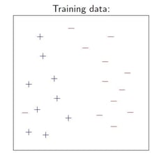
The idea is to find an optimal way to classify our data. To find an optimal algorithm that can classify the images into the mentioned categories. Is it a dog or a cat? We can think of our algorithm like a line that separates our images into two categories. How do we draw this line? Which criteria should we take under consideration? On the pictures below we can see three different ways to separate our data. Three different algorithms.

On the picture on the left we have low training error and a simple classifier. It is simple because it is easy to derive Y from the input X if you think of a linear function (straight line) Y = aX + b. The error is really low since we only got one image wrong.
On the picture in the middle we have again a simple classifier (again a straight line), but our training error is too high since we were not able to divide our data into two groups with same characteristics. Pay attention to the middle picture, we have divided our data into two groups but there is a big error in comparison with the first picture where our data have been classified better. On the last picture now, we have no training error but our classifier is too complex. Imagine the graph of a first degree polynomial is the straight line Y = aX + b. The graph of a second degree polynomial is a curve with function Y = aX2 + bX + c. Imagine now the graph on the last picture which has so many curves... Can you imagine its complexity?
So, for a good training performance we need a good (sufficient, representative and good quality) data, low training error and a simple classifier.

Is your machine best in class?
After selecting the most appropriate algorithm for our case/problem we are ready to score our data. This means based on the training we did in the previous steps, we can see the outcome of it. The machine has learned now and is ready to score the new data. Now we can evaluate our results. How accurate or precise the algorithm was.
What is accuracy and what is precision? Accuracy is simply the proportion of correctly classified instances. It is used to describe how close the measurement to the real value is. Precision is also referred to as a positive predictive value.
In order to understand those two metrics better I am going to use a shooting target example.

On the pictures above, we see two shooting targets. On the picture on the left, we can see that all the four shots were quite close to the center of the target. All the shots were quite accurate but not precise because they were quite far from each other. But on the other picture on the right, we can see that the accuracy is lower because all the shots were far from the center of the target. On the other hand, they were precise since the distance of all four shots is really small.
Back to our case, accuracy is usually the first metric we look at when evaluating a classifier. However, when the test data is unbalanced or we are more interested in the performance, accuracy doesn’t really capture the effectiveness of a classifier. For that reason, it is helpful to compute additional metrics that capture more specific aspects of the evaluation.
When we evaluate our algorithm we focus on the four possible outcomes. The answer to this kind of problems is either Positive or Negative. So, either we predicted that the answer would be Positive and we were correct or wrong (two possible scenarios) or we predicted that the answer would be Negative and we predicted correctly or wrongly (again, two possible scenarios).
So, in total we have four different outcomes. True Positive(TP), False Positive(FP), True Negative(TN) and False Negative(FN). Based on these results we can calculate accuracy/error rate, precision and recall, squared error, etc. I am not going to dive into that in this blog.
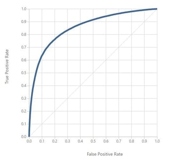
Finally, after calculating the above metrics for choosing our algorithm, we are ready to select the most optimized algorithm. Or even better; the algorithm that describes our data best. The choice of optimization technique is key to the efficiency of the analyst, and also helps determine the classifier produced if the evaluation function has more than one optimum. But do not cultivate fake hopes that the choice of a clever algorithm can have the best results. Better data can defeat a better algorithm!

Predict your numbers so you won’t regret it
The other type of a supervised learning is regression, which is the prediction of a numeric value. We try to estimate real values based on continuous variables. Same concept as in classification. We have a training dataset and then a scoring dataset. Whatever the model has learned from the training set, is being applied to the scoring set. The only difference here is that the algorithm doesn’t provide a class in which your variable will fall, but a numeric value. The evaluation process differs slightly from the evaluation of the classification. This is due to the fact that now we predict a numeric value. In order to evaluate if our algorithm is good enough, we need to know how “far” our predicted value is from the real one. We can measure that using the Mean Absolute Error, Mean Squared Error or the Root Mean Squared Error.
In order to get a better understanding of the concept of regression we can think of it as drawing a trend line over our data, like on the pictures below.
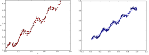
Imagine that this trend line is our algorithm that describes our data. In this specific example, since our algorithm is a straight line, by giving a new data input X, we can predict our output Y by using the function of a straight line Y = aX + b.

Data increasing; models ought to be more capable
Machine learning is already being used in our daily lives even though we may not be aware of it. Examples such as online shopping, Google Adwords, the suggestions Netflix gives what to watch next and many more. When we search to buy a specific product in Amazon for instance, we quickly get a return of a list of the most relevant products. So, the Amazon algorithm quickly learns to combine relevant features in order to give us the product we are looking for.
Although the amount of data coming at us isn’t going to decrease, we are increasingly going to be able to make sense of all this data and it will be an essential skill for people working in a data driven industry to make predictions.
In machine learning, we look at instances of data. Each instance of data is composed of a number of features. By cooking all these features of data we are able to have a glimpse of the future. By choosing the “right” algorithm that best fits our data, we ensure that our results will be helpful and insightful.
So, with more and more data we also need to increase the quality of our models. But do not forget that a dumb algorithm with lots and lots of data beats a clever one with modest amounts of it. So, it’s not always about the choice of the best algorithm but also about the quality and the volume of our data!

See you soon!
Now that we have an almost complete idea about data analysis and how to build a decent predictive model, it would be nice to visualize our findings. Stay tuned for the next blog about the art of the visualization process!
In the meantime, drop me a comment to tell me what’s your view on Machine Learning and creating algorithms.
This blogpost has been translated to Dutch. You can find the Dutch version here.
Written by Agis Christopoulos, Data Scientist at Valid.